

Background
Welcome to Part 4 in the RF Power meter series. Today it’s all about calibration.
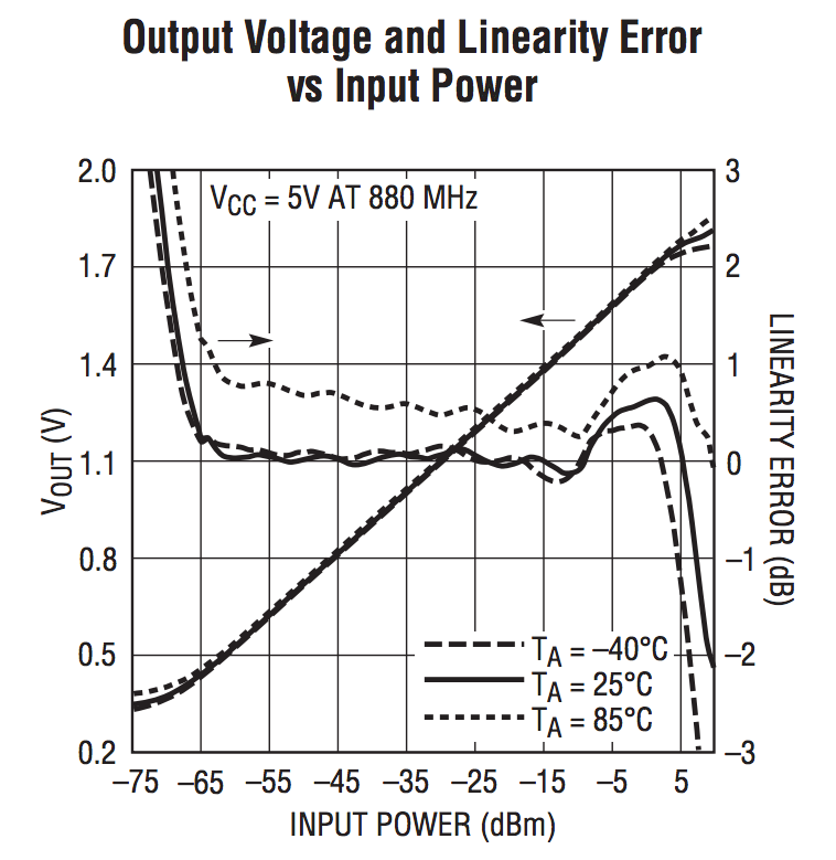
In the original design of the RF Power Meter, I had planned on using slope and intercept values from the datasheet to calculate the displayed RF level. The approach was simple to implement, however, the slope of the graph tended to flatten out at the top and bottom of the range. This would introduce conversion errors with very strong and very weak signal levels. I needed a way to extend the dynamic range of the meter by calibrating out any nonlinearity in the LT5538 analog output.
The way to do that was to introduce a set of calibration tables for each of the six bands.
The table below is taken from the LT5538 specification sheet. It clearly shows the differences, mV/dBm, slope and intercept values for each of the bands.
| Band | Dynamic Range | Slope (mV/dB) | Intercept (dBm) | Sensitivity (dBm) |
|---|---|---|---|---|
| 40 MHz | 76 | 19.9 | -87.3 | -72.0 |
| 450 MHz | 75 | 19.6 | -87.3 | -71.5 |
| 880 MHz | 75 | 19.0 | -88.8 | -71.5 |
| 2140 MHz | 70 | 17.7 | -89.0 | -69.0 |
| 2700 MHz | 65 | 17.6 | -87.5 | -69.5 |
| 3600 MHz | 57 | 18.0 | -81.4 | -63.0 |
Calibration
With the need for calibration tables established, I proceeded to update both the mobile application and the power meter firmware. It also meant that the firmware for the meter could be simplified significantly.
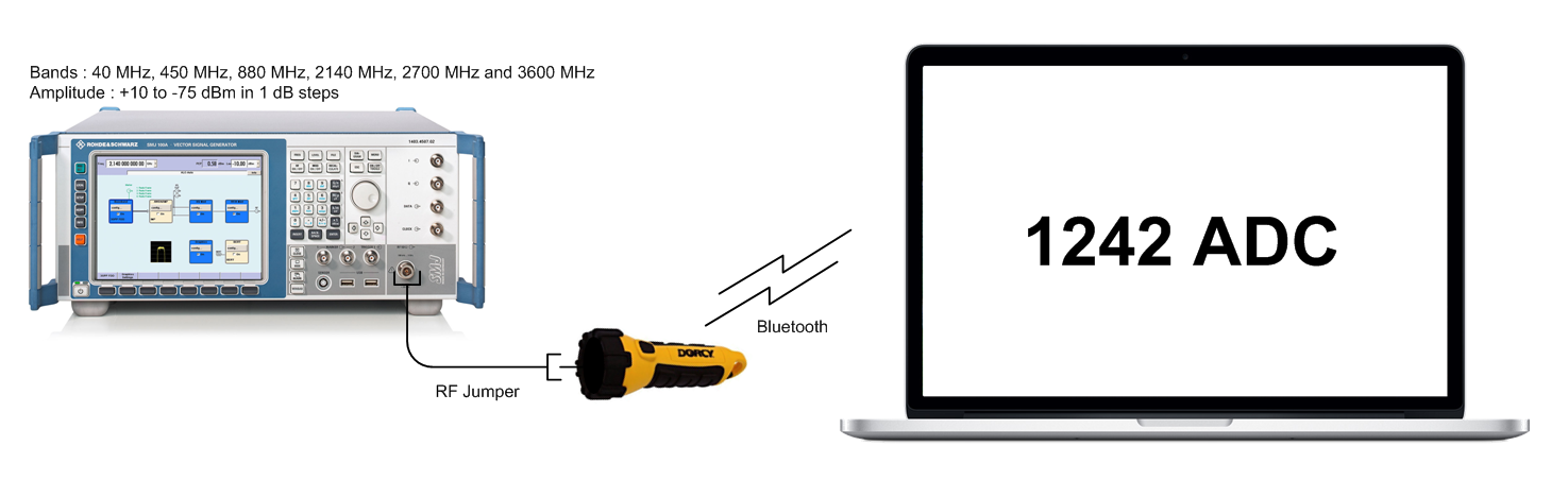 With the original handheld design, the question was how do you provide a calibration process that is easy to implement. With calibration tables, each band required a total of 85 measurements. The original design had four user buttons on the front panel. There was no way to implement a calibration process with just three buttons (the fourth being the power button) that would be both easy and intuitive. Using the flashlight body for the enclosure, allowed me to move the calibration tables and more importantly the entire calibration process to the mobile application. However, this did create a new problem. Would inaccuracies in measurements creep in due to subtle differences in component tolerances? Based on the initial prototypes this did not appear to be an issue.
Mobile Application
In the current prototypes, the calibration data is now stored in the mobile application, not in the actual meter. OK, that’s not entirely true, the meter has a built-in set of calibration tables which get pushed to the mobile application when the meter connects to the application. Any changes or updates to the calibration tables are stored in the mobile application. The updated configuration files are uploaded into the mobile application on all subsequent launches.
The calibration table is an array of 85 values (integers) representing values from +10 dBm to -75 dBm in 1 dB steps. Each array element contains a measurement that is converted by the mobile application into the units to be displayed. The application stores a separate calibration table, for each of the six bands. The actual working range of the meter has been limited from +5 dBm to -70 dBm. Limiting the measurement to a maximum of +5 dBm provides 10 dB of headroom before the power sensor goes up in smoke.

The calibration results are stored in the mobile application as integer values directly from the ADC of the Nordic Semiconductor SOC. The mobile application converts the raw ADC values to dBm using the calibration table based on the selected band. All other units (pW, uW, mW, mV) are then derived from dBm value. The mobile application automatically auto ranges the Watts and Volts units.
Wrap Up
Using calibration tables added complexity to the design but improved the accuracy and extended the operating range of the meter. Calibration tables also allow previously collected data to have new or updated calibration charts applied after the fact. Applying updated calibration tables is useful for “correcting” measurements without having to send staff back into the field to redo the measurements.
That’s it for today. In the next instalment, we’ll cover the mobile application in detail.
That’s it for today. Cheers.